
In March 1990, a Princeton economics professor named Orley Ashenfelter claimed he could predict the quality of a Bordeaux wine without tasting it.
All he needed was the vintage's age and some weather data: the temperature and rainfall of the year the grapes grew.
The wine world didn't take it well. Robert Parker, the most influential critic of the time, called Ashenfelter "an absolute total sham" and compared him to a movie critic who never sees the movie but tells you how good it is based on the actors and the director.
Then came the predictions. Parker rated the 1986 vintage "very good to sometimes exceptional". Ashenfelter thought it was mediocre. And he declared that 1989 would be "the wine of the century", and that 1990 would be even better.
At auction, the 1989 vintage went on to sell for more than twice the price of the 1986. The 1990 sold for even more.
The tool behind these predictions is one of the simplest in statistics: linear regression. In this article, we'll rebuild Ashenfelter's model in Python, with the original data, and see what it teaches us about making decisions with data.
Linear regression in one sentence
Linear regression finds the line that passes closest to a set of points.
On one side is what we want to predict, the dependent variable: here, the price of the wine. On the other are the independent variables, which we use to make the prediction: temperature, rain, age.
With a single variable, you can see the idea in a chart. Each point below is a Bordeaux vintage, between 1952 and 1978:
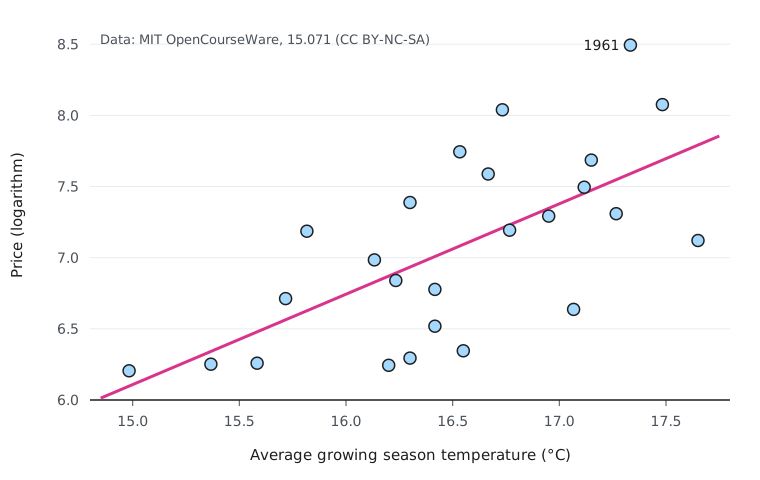
The trend is clear: warmer years make pricier wines. The magenta line is the one the regression picked: out of all possible lines, it's the one with the smallest sum of squared errors, that is, the smallest total distance to the points.
But notice that many points sit far from the line. Temperature explains part of the story, not all of it.
To measure how much it explains, we use R². It goes from 0 to 1:
- 0 means the model is no better than guessing the average price for every vintage;
- 1 means the model gets everything right.
Temperature alone has an R² of 0.44: it explains 44% of the price variation between vintages.
Hands-on: the model in Python
The data Ashenfelter used is available in MIT OpenCourseWare's The Analytics Edge course, which uses this case to teach regression. We'll need two libraries:
pip install pandas statsmodelsThe course splits the data into two files: 25 vintages (1952 to 1978) to build the model, and 2 vintages (1979 and 1980) set aside to test it later.
import pandas as pd
import statsmodels.formula.api as smf

MIT = "https://ocw.mit.edu/courses/15-071-the-analytics-edge-spring-2017/"
vintages = pd.read_csv(MIT + "e6eb689583a501e5b4c6164d771880d9_wine.csv")
new_vintages = pd.read_csv(MIT + "fbf05b0e868bc87b4fbadac6fe406c30_wine_test.csv")

print(vintages.head())
Each row is a vintage, with these columns:
| Column | What it is |
|---|---|
Price | Typical price of the vintage at 1990 and 1991 auctions, as a logarithm |
AGST | Average temperature during the grape growing season (°C) |
HarvestRain | Rain around harvest time (mm) |
WinterRain | Rain in the preceding winter (mm) |
Age | Age of the vintage (years) |
FrancePop | Population of France in the vintage year (thousands) |
The price comes as a logarithm because wine prices vary enormously between vintages: one can be worth ten times another. On a log scale, the relationship with the weather gets closer to a straight line, and each coefficient becomes a percentage change, as we'll see.
First, the model from the chart, with temperature only:
model_1 = smf.ols("Price ~ AGST", data=vintages).fit()
print(round(model_1.rsquared, 2))  # 0.44
The formula "Price ~ AGST" reads as "price as a function of temperature". To use more variables, just add them:
model = smf.ols("Price ~ AGST + HarvestRain + Age + WinterRain", data=vintages).fit()
print(round(model.rsquared, 2))  # 0.83
print(model.params)
Each variable added raises the R²:
| Variables | R² |
|---|---|
| Temperature | 0.44 |
| + harvest rain | 0.71 |
| + age | 0.79 |
| + winter rain | 0.83 |
With four numbers about the weather and the age, the model explains 83% of the price variation between vintages. Without tasting a drop.
To see the full report, with standard errors and significance tests, use print(model.summary()).
Reading the coefficients
model.params shows how much each variable weighs:
Intercept     -3.429980
AGST           0.607209
HarvestRain   -0.003972
Age            0.023931
WinterRain     0.001076
Because the price is a logarithm, each coefficient translates into a percentage change. The math is exp(coefficient × change) − 1, and the result looks like this:
| If... | the vintage's price... |
|---|---|
| the growing season is 1 °C warmer | rises about 84% |
| it rains 100 mm more at harvest | falls about 33% |
| it rains 100 mm more in winter | rises about 11% |
| the vintage is 1 year older | rises about 2.4% |
All of this holds the other variables constant, and it makes sense to anyone who knows grapes: a hot summer ripens the fruit, rain at harvest dilutes the juice, winter rain fills the soil for the growing season, and wine made to age gains value over time.
This is one of linear regression's great strengths: the model can be read and discussed. It's not a black box. A winemaker can look at this table and decide whether they agree.
The real test: vintages the model never saw
An R² of 0.83 looks great, but it measures accuracy on the same vintages used to build the model. It's like grading your own exam.
The test that matters uses new data. That's what the 1979 and 1980 vintages are for:
def out_of_sample_r2(model, new_vintages, vintages):
    predicted = model.predict(new_vintages)
    model_error = ((new_vintages.Price - predicted) ** 2).sum()
    baseline_error = ((new_vintages.Price - vintages.Price.mean()) ** 2).sum()
    return 1 - model_error / baseline_error

print(round(out_of_sample_r2(model, new_vintages, vintages), 2))  # 0.79
Repeating the test for each combination of variables:
| Variables | R² on the 25 vintages | R² on the 2 new vintages |
|---|---|---|
| Temperature | 0.44 | 0.79 |
| + harvest rain | 0.71 | −0.08 |
| + age | 0.79 | 0.53 |
| + winter rain | 0.83 | 0.79 |
| + population of France | 0.83 | 0.76 |
Two lessons come out of this table:
- A better fit doesn't guarantee a better prediction. The model with temperature and harvest rain rises to 0.71 on the training data, but does worse than the average on the new vintages: its R² goes negative, which can only happen out of sample.
- Two vintages are far too few to conclude anything. With a sample that small, a single unusual year changes everything. The MIT course itself makes this point.
Before you trust the model
Correlation isn't causation. Look at the last row of the table: the population of France. On its own, it has an R² of 0.22 with the price of wine. The French don't make wine pricier by being born: the population grew year after year, so it moves together with the vintage's age (the correlation between the two is −0.99). The regression doesn't know that. You need to.
Little data, double the care. There are 25 vintages. Each extra variable is one more number the model has to estimate from the same small amount of information. That's what happened with the population of France: it didn't improve the R², and it made the test worse.
Don't extrapolate. The data runs from 15 to 17.7 °C. The model doesn't know what happens in a 20 °C summer, and the line surely doesn't keep rising forever: too much heat ruins grapes too.
Not every relationship is a straight line. Linear regression assumes each extra degree has the same effect. When that doesn't hold, it's time to transform the variables, as we did with the logarithm of the price, or to use another model.
Why this is about decisions
Ashenfelter's story isn't about wine. It's about what happens when a simple, transparent model meets expert opinion.
The model didn't replace anyone's palate. It did something more useful: it gave winemakers and buyers an early, objective and verifiable estimate, in a market where a vintage's quality only becomes clear after years in the bottle.
That's the best way to think about data for decisions: before any sophisticated model, ask which few variables explain most of the problem, and test that answer on data the model has never seen.